"You will can get notification in to your G mail ,when we are upload our new article . so you can follow this blog site. you can see "blank line" on the top line of the blog page, type your gmail and then submit. "
Direct costs and indirect costs
Costs may be classified as direct costs or indirect costs. The purpose of this classification is to assign costs to cost objects. Cost object means any thing about which cost information is collected. Some examples of cost objects are products, departments, customers, plant, a territory, a product line and research and development activities of the business etc.
A brief explanation of direct costs and indirect costs are given below:
Direct cost:
A cost that is easily traceable to a particular cost object is known as direct cost. The use of the term “direct cost” is not limited to direct materials and direct labor. Every cost that can be easily and conveniently traced to a particular product, customer, branch, plant or any other cost object is a direct cost. For example, if Bata shoes company wants to assign costs to all the branches in Pakistan, then the salary of the manager of Islamabad branch would be a direct cost of that branch
Indirect cost:
A cost that is not easily traceable to a particular cost object is called indirect cost. For example, a clothing factory produces different varieties of cloths. The salary of the manager would be an indirect cost because it is caused by all the varieties and is not easily traceable to a particular variety. The Rafhan Maize Products company produces a large number of products by processing tones of corn every year. The salary of the factory manager is an indirect cost for the products because it is not caused by a particular product.
The costs that are caused by a number of cost objects but cannot be traced to a particular cost object is known as common cost. In our examples, the salaries of the managers of clothing factory and Rafhan maize products are common costs.
When we say direct or indirect cost, we mean that it is direct or indirect with respect to a particular cost object. A cost may be direct for one cost object but indirect for another. For example, National Food Products Co. has a number of branches in Pakistan. Each branch sells a variety of food products. The salary of the manager of Karachi branch would be an indirect cost of a particular product but direct cost of the branch as a whole.
Variable, fixed and mixed (semi-variable) costs
As the level of business activities changes, some costs change while others do not. The response of a cost to a change in business activity is known as cost behavior. Managers should be able to predict the behavior of a particular cost in response to a change in particular business activity. For this purpose, costs are classified as variable, fixed and mixed costs. This article explains these three types of costs as well as their response to business activities.
Variable cost:
A cost that changes, in total dollar amount, with the change in the level of activity is called variable cost. A common example of variable cost is direct materials cost. Consider the following example to understand how variable cost behaves in a manufacturing company.
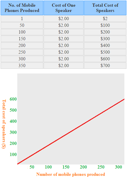
A mobile phone manufacturing company purchases speakers from another company at a cost of $2 per speaker. The speaker is a direct materials cost for mobile phone manufacturing company. One speaker is used to complete a mobile phone. The total and per unit cost of speakers at various levels of activity is given below:
Notice that the total cost of speakers increases as the mobile phones produced are increased but per unit cost remains constant.
Other examples of variable cost include lubricants, sales commission and shipping costs etc
Fixed cost:
A cost that does not change, in total, with the change in activity is called fixed cost. A common example of fixed cost is rent. In above example, if mobile phone manufacturing company rents a building for its factory for $5,000 per month, it will have to pay $5,000 for every month even no mobile phone is produced during the month. The behavior of fixed cost is shown in the following figure:
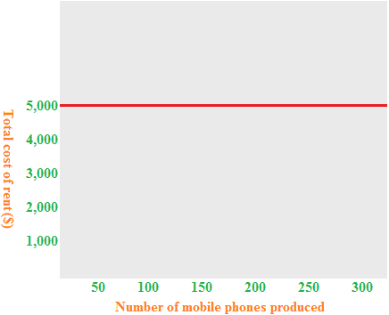
Total fixed cost does not change with the change in activity but per unit fixed cost changes with the rise and fall in the level of activity. There is an inverse relationship between per unit fixed cost and activity. If production increases, per unit fixed cost decreases and if production decreases, per unit fixed cost increases. To understand this point, we can use the data from the above example of mobile manufacturing company. Consider the following table:
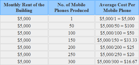
Notice that average fixed cost (computed in the last column) decreases as the production of mobile phones increases. It is an interesting property of fixed cost.
Mixed or semi-variable cost:
A cost that has the characteristics of both variable and fixed cost is called mixed or semi-variable cost. For example, the rental charges of a machine might include $500 per month plus $5 per hour of use. The $500 per month is a fixed cost and $5 per hour is a variable cost. Another example of mixed or semi-variable cost is electricity bill. The electricity bill can be divided into two parts – (1) line rent and (2) cost of units consumed. The line rent is not affected by the consumption of electricity whereas the cost of units consumed varies with the change in units consumed.
Three commonly used methods to divided a mixed or semi-variable cost into its fixed and variable components are high-low point method, scatter graph method and least squares regression method.
Product costs and period costs
Costs may be classified as product costs and period costs. This classification is usually used for financial accounting purposes. A brief explanation of product costs and period costs is given below:
Product costs:
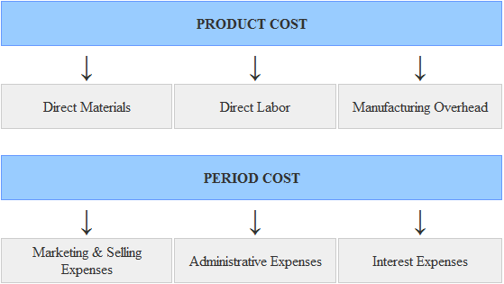
Product costs (also known as inventoriable costs) are those costs that are incurred to acquire or manufacture a product. For a manufacturing company, theses costs usually consist of direct materials, direct labor, and manufacturing overhead.
Product costs are initially treated as inventory and do not appear on income statement until the product for which they are incurred is sold. When the product is sold, these costs are transferred to cost of goods sold account. For example, John & Muller company manufactures 50 units of product X in year 2020. Out of these 50 units manufactured, the company sells only 30 units during the year and 20 unsold units remain as ending inventory. The direct materials, direct labor and manufacturing overhead costs incurred to manufacture these 50 units will be initially treated as inventory (i.e., an asset). The inventory of 30 units will be transferred to cost of goods sold during the year 2020 and appear on the income statement of 2020. The remaining inventory of 20 units will not be transferred to cost of good sold in 2020 but will be listed as current asset in the John & Muller’s balance sheet. These unsold units will continue to be treated as asset until they are sold next year and their cost is transferred to cost of goods sold account.
Period costs:
The costs that are not included in product costs are known as period costs. Usually, these costs are not part of the manufacturing process and are therefore treated as expense for the period in which they arise.
Period costs are not attached to products and company does not need to wait for the sale of its products to recognize them as expense. According to generally accepted accounting principles (GAAP), all marketing, selling and administration costs are treated as period costs. Examples of these costs include office rent, interest, depreciation of office building, sales commission and advertising expenses etc.
A summary of the concepts explained above is given below:
Manufacturing and non-manufacturing costs
Costs may be classified as manufacturing costs and non-manufacturing costs. This classification is usually used by manufacturing companies.
Manufacturing costs:
Manufacturing costs can be further divided into the following categories:
- Direct materials
- Direct labor
- Manufacturing overhead
The above three categories of manufacturing costs are briefly explained below:
Direct materials:
Materials that become an integral part of the finished product and that can be easily traced to it are called direct materials. For example wood is a direct material for the manufacturers of furniture. Lime stone is direct material for the manufacturers of cement. Direct materials usually consists of a significant portion of total manufacturing cost. Direct material is sometime called raw material.
The finished product of a company may become raw material of another company. For example, cement is a finished product for manufacturers of cement and raw materials for companies involved in construction business.
Direct labor:
The labor cost that can be physically and conveniently traced to a unit of finished product is called direct labor cost or touch labor cost. Examples of direct labor cost include labor cost of machine operators and painters in a manufacturing company. Like direct materials, it comprises of a significant portion of total manufacturing cost.
The sum of direct materials cost and direct labor cost is known as prime cost.
Formula of prime cost:
Prime cost = Direct materials cost + Direct labor cost
Manufacturing overhead cost:
Manufacturing costs other than direct materials and direct labor are categorized as manufacturing overhead cost (also known as factory overhead costs). It usually includes indirect materials, indirect labor, salary of supervisor, lighting, heat and insurance cost of factory etc. Usually, manufacturing overhead costs cannot be easily traced to individual units of finished products.
The sum of direct labor cost and manufacturing overhead cost is known as conversion cost.
Formula of conversion cost:
Conversion cost = Direct labor cost + Manufacturing overhead cost
The sum of direct materials cost, direct labor cost and manufacturing overhead cost is known as manufacturing cost.
Formula of manufacturing cost:
Manufacturing cost = Direct materials cost + Direct labor cost + Manufacturing overhead cost
Non-manufacturing costs:
Non-manufacturing costs are further divided into the following categories:
- Marketing and selling costs
- Administrative costs
Examples of marketing and selling costs include advertising costs, order taking costs and salaries of sales persons etc. Examples of administrative costs include salaries of executives, accounting costs, and general administration costs etc.
Differential, opportunity and sunk costs
Differential cost:
The work of managers includes comparison of costs and revenues of different alternatives. Differential cost (also known as incremental cost) is the difference in cost of two alternatives. For example, if the cost of alternative A is $10,000 per year and the cost of alternative B is $8,000 per year. The difference of $2,000 would be differential cost. The differential cost can be a fixed cost or variable cost.
Similarly the difference in revenue of two alternatives is known as differential revenue. For example, if alternative A’s revenue is $15,000 and alternative B’s revenue is $10,000. The difference of $5,000 would be differential revenue.
When different revenue generating alternatives are compared, the differential cost as well as differential revenues associated with each alternative is taken into account.
The terms “differential cost” and “differential revenue” used in managerial accounting are similar to the terms “marginal cost” and “marginal revenue” used in economics.
Example – computation of differential cost, differential revenues and differential net operating income:
The management of Galaxy company has two alternatives to choose from. Compute differential revenue, differential cost and differential net operating income from the information of two alternatives given below:
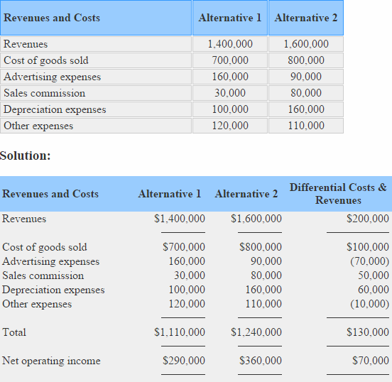
In the above example, total differential revenue is $200,000 (1,600,000 – 1,400,000), differential cost is $130,000 (1,240,000 – 1,110,000) and differential net operating income is $70,000 ($360,000 – $290,000).
If a decision is made on the basis of above computations, alternative 2 would be selected because it promises to generate more net operating income.
Opportunity cost:
Unlike other types of cost, opportunity cost does not require the payment of cash or its equivalent. It is a potential benefit or income that is given up as a result of selecting an alternative over another. For example, You have a job in a company that pays you $25,000 per year. For a better future, you want to get a Master’s degree but cannot continue your job while studying. If you decide to give up your job and return to school to earn a Master’s degree, you would not receive $25,000. Your opportunity cost would be $25,000.
Almost every alternative has an opportunity cost. It is not entered in the accounting records but must be considered while making decisions.
Sunk cost:
The costs that have already been incurred and cannot be changed by any decision are known as sunk costs. For example, a company purchased a machine several years ago. Due to change in fashion in several years, the products produced by the machine cannot be sold to customers. Therefore the machine is now useless or obsolete. The price originally paid to purchase the machine cannot be recovered by any action and is therefore a sunk cost.
These costs should not be taken into account while making any decision because no action can revers them.
Treatment of idle time, overtime premium, and fringe benefit costs
Treatment of idle time:
Idle time means the amount of time the workers remain idle in a normal working day. The idle time is usually caused by a sudden fault in machine or equipment, power failure, lack of orders for the product, inefficient work scheduling, defective materials and shortage of raw materials etc. The cost associated with idle time is treated as indirect labor cost and should, therefore, be included in manufacturing overhead cost. For example, the normal weekly working hours of a worker are 48 and he is paid @ $8 per hour. If he remains idle for 6 hours due to power failure, then the cost of 42 hours would be treated as direct labor cost and the cost of 6 hours (idle time) would be treated as indirect labor cost and included in manufacturing overhead cost.

Treatment of overtime premium:
Overtime premium is the amount that is paid, for the overtime worked, in excess of the normal wage rate. Like idle time, overtime premium is also treated as indirect labor cost and included in manufacturing overhead cost. For example, a worker normally works for 48 hours per week @ $8 per hour. In a particular week, if he works for 52 hours and company pays him $12 for every hour worked in excess of 48 hours, the allocation of the labor cost of the worker would be made as follows:

The amount of $16 is overtime premium and is a part of manufacturing overhead cost.
Treatment of labor fringe benefits:
Fringe benefits are benefits that employers provide to employees in addition to normal salaries or wages. Examples of fringe benefits are hospitalization, insurance programs, retirement plans, paid holidays and stock options etc. Most of the companies treat labor fringe benefits as indirect labor and, therefore, include them in manufacturing overhead costs.
A few firms treat direct labor related fringe benefits as addition to direct labor cost which is considered a more superior practice.
The above information has been summarized below:
Costs of quality or quality costs
Costs of quality or quality costs does not mean the use of expensive or very highly quality materials to manufacture a product. The term refers to the costs that are incurred to prevent, detect and remove defects from products. Quality costs are categorized into four main types. Theses are:
- Prevention costs
- Appraisal costs
- Internal failure costs and
- External failure costs.
These four types of quality costs are briefly explained below:
Prevention costs:
It is much better to prevent defects rather than finding and removing them from products. The costs incurred to avoid or minimize the number of defects at first place are known as prevention costs. Some examples of prevention costs are improvement of manufacturing processes, workers training, quality engineering, statistical process control etc.
Appraisal costs:
Appraisal costs (also known as inspection costs) are those cost that are incurred to identify defective products before they are shipped to customers. All costs associated with the activities that are performed during manufacturing processes to ensure required quality standards are also included in this category. Identification of defective products involve the maintaining a team of inspectors. It may be very costly for some organizations.
Internal failure costs:
Internal failure costs are those costs that are incurred to remove defects from the products before shipping them to customers. Examples of internal failure costs include cost of rework, rejected products, scrap etc.
External failure costs:
If defective products have been shipped to customers, external failure costs arise. External failure costs include warranties, replacements, lost sales because of bad reputation, payment for damages arising from the use of defective products etc. The shipment of defective products can dissatisfy customers, damage goodwill and reduce sales and profits.
More examples of quality costs
Examples of prevention cost
- System development
- Quality engineering
- Quality training
- Quality circles
- Statistical process control
- Supervision of prevention
- Quality improvement projects
- Technical support to suppliers
- Quality data gathering, analysis and reporting
- Audit of the quality system
Examples of appraisal cost
- Test and inspection of incoming materials
- Final product testing and inspection
- Supplies used in testing and inspection
- Supervision of testing and inspecting activities
- Depreciation of test equipment
- Maintenance of test equipment
- Plant utilities in inspection area
- Field testing and appraisal at customer site
Examples of internal failure cost
- Net cost of scrap
- Net cost of spoilage
- Rework labor and overhead
- Reinspection of reworked products
- Disposal of defective products
- Down time caused by quality problems
- Analysis of the cause of defects in the production
- Retesting of reworked products
- Re-entering data because of keying
- Debugging software errors
Examples of external failure cost
- Cost of field servicing and handling complaints
- Warranty repairs and replacement costs
- Liability arising from defective products
- Lost sales arising from a reputation of poor quality
- Returns and allowances arising from quality problems
- Product recalls
- Repairs and replacements beyond the warranty period
High-low point method
High-low point method is a technique used to divide a mixed cost into its variable and fixed components.
Sometimes it is necessary to determine the fixed and variable components of a mixed cost figure. Several techniques are used for this purpose such as scatter graph method, least squares regression method and high-low point method. On this page I will explain the use of high-low point method.
Under high-low point method, an estimated variable cost rate is calculated first using the highest and lowest activity levels and mixed costs associated with them. This estimated variable cost rate is used to calculate total estimated variable cost included in the mixed cost figures at highest and lowest activity levels. The estimated variable cost is then subtracted from the total mixed cost figures at highest and lowest activity levels to find the fixed cost component.
The cost function
Like scatter graph method and least squares regression method, high-low point method follows the following cost function (also known as cost volume formula):
y = a + bx
Where,
- y = total cost
- a = total fixed cost
- b = fixed cost
- x = number of units
To make the procedure simple and easy to understand , we can divide the calculations into the following three steps.
Steps involved in high-low point method
Step 1 – calculation of variable cost rate:
The first step in high-low point method is to calculate an estimated variable cost rate. This rate is calculated by using the following formula:

Step 2 – calculation of variable cost component:
After calculating estimated variable cost rate, the second step is to calculate the total estimated variable cost at highest and lowest activity levels. It is calculated by multiplying the estimated variable cost rate (calculated in step 1) by highest and lowest activity levels. The formula is given below:
Estimated total variable cost = Estimated variable cost rate × Highest or lowest level of activity
Step 3 – calculation of fixed cost component:
The third and final step in high-low point method is to find out the fixed cost component of the total mixed cost. It is calculated by subtracting the estimated variable cost (calculated in step 2) from the total mixed cost figure. The formula for this purpose is given below:
Fixed cost = Total mixed cost – Estimated total variable
Example:
The Western Company presents the production and cost data for the first six months of the 2015.

Required: Determine the estimated variable cost rate and fixed cost using high-low point method. Also determine the cost function on the basis of data given above.
Solution:
Variable cost rate
(66,000 – 45,000)/(29,000 – 15,000)
= $21000/14,000
= $1.5 per unit
Variable cost:
- Highest activity level (May): 29,000 units × $1.5 = $43,500
- Lowest activity level (January): 15,000 × $1.5 = $22,500
Fixed cost:
- Highest activity level (May): $66,000 – $43,500 = $22,500
- Lowest activity level (January): $45,000 – $22,500 = $22,500
On the basis of data provided by Western Company, the cost function is:
y = $22,500 + $1.5x
The high-low point method uses only two data points (the highest and the lowest activity levels). Therefore, It is considered a less reliable method as compared to other methods available for mixed cost analysis
Least squares regression method
Definition and explanation
Least squares regression method is a method to segregate fixed cost and variable cost components from a mixed cost figure. It is also known as linear regression analysis.
Least squares regression analysis or linear regression method is deemed to be the most accurate and reliable method to divide the company’s mixed cost into its fixed and variable cost components. This is because this method takes into account all the data points plotted on a graph at all activity levels which theoretically draws a best fit line of regression.
Linear regression is basically a mathematical analysis method which considers the relationship between all the data points in a simulation. All these points are based upon two unknown variables; one independent and one dependent. The dependent variable will be plotted on the y-axis and the independent variable will be plotted to the x-axis on the graph of regression analysis. In literal manner, least square method of regression minimizes the sum of squares of errors that could be made based upon the relevant equation.
The least squares regression method follows the same cost function as the other methods used to segregate a mixed or semi variable cost into its fixed and variable components. Let’s assume that the activity level varies along x-axis and the cost varies along y-axis. The following equation should represent the the required cost line:
y = a + bx
Where,
- y = total cost
- a = total fixed cost
- b = fixed cost
- x = number of units
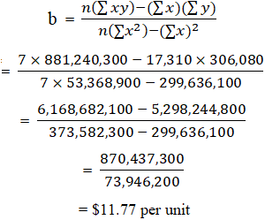
The values of ‘a’ and ‘b’ may be found using the following formulas.
Example
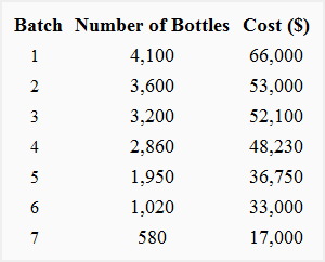
For example, Master Chemicals produces bottles of a cleaning lubricant. The activity levels and the attached costs are shown below:
Required: On the basis of above data, determine the cost function using the least squares regression method and calculate the total cost at activity levels of 6,000 and 10,000 bottles.
Solution
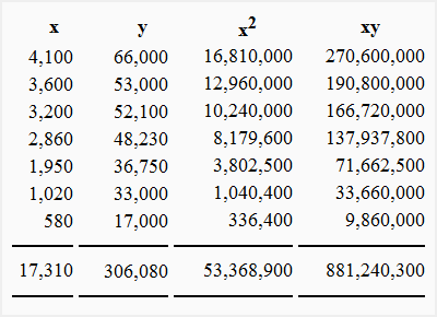
In our example:
- n = 7
- ∑x = 17,310
- ∑y = 306,080
- x2 = 53,368,900
- xy = 881,240,300
We can find the values of ‘a’ and ‘b’ by putting this information in the above formulas:
Computation of variable cost per unit (b):
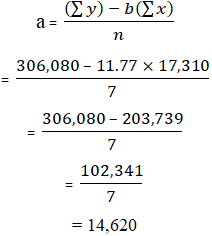
The value of ‘b’ (i.e., per unit variable cost) is $11.77 which can be substituted in fixed cost formula to find the value of ‘a’ (i.e., the total fixed cost).
Computation of total fixed cost (a):
1. Using the method of least squares, the cost function of Master Chemicals is:
y = $14,620 + $11.77x
2. The total cost at an activity level of 6,000 bottles:
y = $14,620 + ($11.77 × 6,000)
= $85,240
3. The total cost at an activity level of 12,000 bottles:
y = $14,620 + ($11.77 × 12,000)
= $155,860
Limitations of least squares regression method:
This method suffers from the following limitations:
- The least squares regression method may become difficult to apply if large amount of data is involved thus is prone to errors.
- The results obtained are based on past data which makes them more skeptical than realistic.
Scatter graph method
Definition and explanation
Scatter graph method is a visual representation used to divide fixed and variable cost components from a mixed cost figure. This is done by plotting the points at which the cost on one axis and activity on another axis meet to find out the correlation between these two variable.
Scatter graph method makes use of a graphical representation of ‘mixed cost’ of a company and the activity levels which affect this cost or due to which this cost is incurred. The activity levels of the business is usually marked upon the horizontal axis (i.e., x-axis) and the attached costs on the vertical axis (i..e., y-axis). A regression line is then drawn to match the points at which these two variables meet.
Like high-low point method and least squares regression method of mixed cost analysis, scatter graph method follows the following cost function:
y = a + bx
Where:
- y = total cost
- a = total fixed cost
- b = variable cost units
- x = activity level
Steps involved in analysis of mixed cost using scatter graph method:
- Different points are marked on the graph for the costs incurred at different activity levels. The x-axis is usually used for activity and y-axis for costs.
- A regression line is carefully drawn to match the data points to find out the relationship between the two variables. Try should be made to minimize the vertical distance between the data points and the regression line while drawing the line through visual inspection. For mixed cost, the line will usually start from an upper point on y-axis rather than from the pivot point which would indicate the presence of fixed cost element. The slope or upward slant of the line shows a gradual increase in the cost with increasing activity level. It indicates the presence of variable cost element in the total cost.
- After determining the total fixed cost in step 2, the slope of the regression line (i.e., variable cost per unit) is calculated by using two points (x1, y1) and (x2, y2) on the line. The formula to find per unit variable cost can be written as follows:
Example
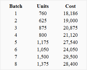
The Cannon Company provides you the following overhead cost data for eight production runs.
Required: Determine the cost function from the data provided by Cannon Company using scatter graph method of mixed cost analysis.
Solution
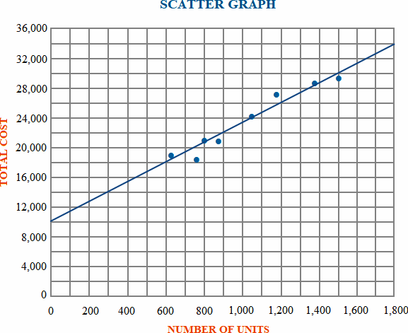
For the above scatter graph, the activity level or production in units is presented on x-axis and the related costs are presented on y-axis. A regression line is drawn which extends from left to right to show an increase in cost as the level of activity increases.
As can be seen the costs are not plotted from ‘O’ the pivot point, but from an upper point, which shows that at zero activity level there exists a cost of $10,000. This is the point where regression line cuts y-axis and which represents the total fixed cost of $10,000. The slop of the regression line (i.e., variable cost per unit) can be found out as follows:
Variable cost per unit = (y2 – y1)/(x2 – x1)
= (34,000 – 10,000)/(1,800 – 0)
= 24,000/1,800
= $13.33
The cost function on the basis of data provided by Cannon Company is as follows:
y = $10,000 + $13.33x
Limitations:
The results obtained from scatter graph approach are not ideal. The main reasons for this are as follows:
- The line or curve plotted on the graph only shows an estimate of the cost which may or may not be close to the real cost.
- This method cannot be used to estimate the segregation of mixed cost where step-costing (the increase in the level of fixed cost after a certain level) is used.
click the follow button in this blog site, comment your ideas, and like to page and subscribe to our official YouTube channel
Thank you.
FOLLOW US.
Presenting by -Accounting way
for more information -
follow "accounting way" official face book accoun
